```{r}
library(datasets)

data(airquality)
```Introduction:
Data wrangling is a crucial step in the data analysis process, and R provides a powerful set of tools and packages to help you clean, transform, and prepare your data for analysis. In this blog post, we will explore some best practices for effective data wrangling in R. Whether you are a beginner or an experienced data analyst, these tips will help you streamline your data preparation workflow and ensure the reliability of your analysis.
Now continuing from the previous post (Best Practices for Data Wrangling in R - Part 1), we will use the airquality data from datasets library to further understand how data wrangling helps us to get the deeper and significant insights of our data.
Reading Data
Raw Input Data
Firstly read your data into R. For this exercise I will be using a simulated dataset.
Understand Your Data
It’s imperative to have a thorough understanding of your dataset before getting started with data wrangling. Knowing your data’s structure, the significance of each variable, and any potential problems or abnormalities is part of this. To obtain an understanding of the data you’re working with, start by analyzing it using functions like head(), summary(), and str().
```{r}
# Example: Inspect the first few rows of a dataset
head(airquality)
```Ozone <int> | Solar.R <int> | Wind <dbl> | Temp <int> | Month <int> | Day <int> | |
|---|---|---|---|---|---|---|
| 1 | 41 | 190 | 7.4 | 67 | 5 | 1 |
| 2 | 36 | 118 | 8.0 | 72 | 5 | 2 |
| 3 | 12 | 149 | 12.6 | 74 | 5 | 3 |
| 4 | 18 | 313 | 11.5 | 62 | 5 | 4 |
| 5 | NA | NA | 14.3 | 56 | 5 | 5 |
| 6 | 28 | NA | 14.9 | 66 | 5 | 6 |
```{r}
# Example: Get a summary of the dataset
summary(airquality)
```
Ozone Solar.R Wind Temp
Min. : 1.00 Min. : 7.0 Min. : 1.700 Min. :56.00
1st Qu.: 18.00 1st Qu.:115.8 1st Qu.: 7.400 1st Qu.:72.00
Median : 31.50 Median :205.0 Median : 9.700 Median :79.00
Mean : 42.13 Mean :185.9 Mean : 9.958 Mean :77.88
3rd Qu.: 63.25 3rd Qu.:258.8 3rd Qu.:11.500 3rd Qu.:85.00
Max. :168.00 Max. :334.0 Max. :20.700 Max. :97.00
NA's :37 NA's :7
Month Day
Min. :5.000 Min. : 1.0
1st Qu.:6.000 1st Qu.: 8.0
Median :7.000 Median :16.0
Mean :6.993 Mean :15.8
3rd Qu.:8.000 3rd Qu.:23.0
Max. :9.000 Max. :31.0
```{r}
# Example: Display the structure of the dataset
str(airquality)
```
'data.frame': 153 obs. of 6 variables:
$ Ozone : int 41 36 12 18 NA 28 23 19 8 NA ...
$ Solar.R: int 190 118 149 313 NA NA 299 99 19 194 ...
$ Wind : num 7.4 8 12.6 11.5 14.3 14.9 8.6 13.8 20.1 8.6 ...
$ Temp : int 67 72 74 62 56 66 65 59 61 69 ...
$ Month : int 5 5 5 5 5 5 5 5 5 5 ...
$ Day : int 1 2 3 4 5 6 7 8 9 10 ...This will help you make informed decisions during the wrangling process.
Data Cleaning
Data cleaning involves checking the headers, handling missing values, outliers, and errors in your dataset. Here are some best practices for data cleaning in R:
Handle Missing Values:
Identify missing values using functions like
is.na()orcomplete.cases().Decide whether to impute missing values, remove rows with missing data, or keep them, depending on the context.
Use packages like
dplyrortidyrto perform missing data operations.
```{r}
library(dplyr)
library(tidyr)

# Example: Remove rows with missing values
airquality_clean <- na.omit(airquality)

head(airquality_clean)
```Ozone <int> | Solar.R <int> | Wind <dbl> | Temp <int> | Month <int> | Day <int> | |
|---|---|---|---|---|---|---|
| 1 | 41 | 190 | 7.4 | 67 | 5 | 1 |
| 2 | 36 | 118 | 8.0 | 72 | 5 | 2 |
| 3 | 12 | 149 | 12.6 | 74 | 5 | 3 |
| 4 | 18 | 313 | 11.5 | 62 | 5 | 4 |
| 7 | 23 | 299 | 8.6 | 65 | 5 | 7 |
| 8 | 19 | 99 | 13.8 | 59 | 5 | 8 |
Other methods to remove NA’s include na.omit() , complete.cases(), rowSums(), drop_na(), and filter().
```{r}
# #Remove rows with NA's using na.omit()
# airquality_clean <- na.omit(airquality)
#
# #Remove rows with NA's using complete.cases
# airquality_clean <- airquality[complete.cases(airquality),]
#
# #Remove rows with NA's using rowSums()
# airquality_clean <- airquality[rowSums(is.na(airquality)) == 0,]
#
# #Import the tidyr package
# library("tidyr")
#
# #Remove rows with NA's using drop_na()
# airquality_clean <- airquality %>% drop_na()
#
# #Remove rows that contains all NA's
# airquality_clean <-
# airquality[rowSums(is.na(airquality)) != ncol(airquality),]
#
# #Load the dplyr package
# library("dplyr")
#
# #Remove rows that contains all NA's
# airquality_clean <-
# filter(airquality, rowSums(is.na(airquality)) != ncol(airquality))
#
# airquality_clean <- airquality %>% filter(!is.na(Ozone))
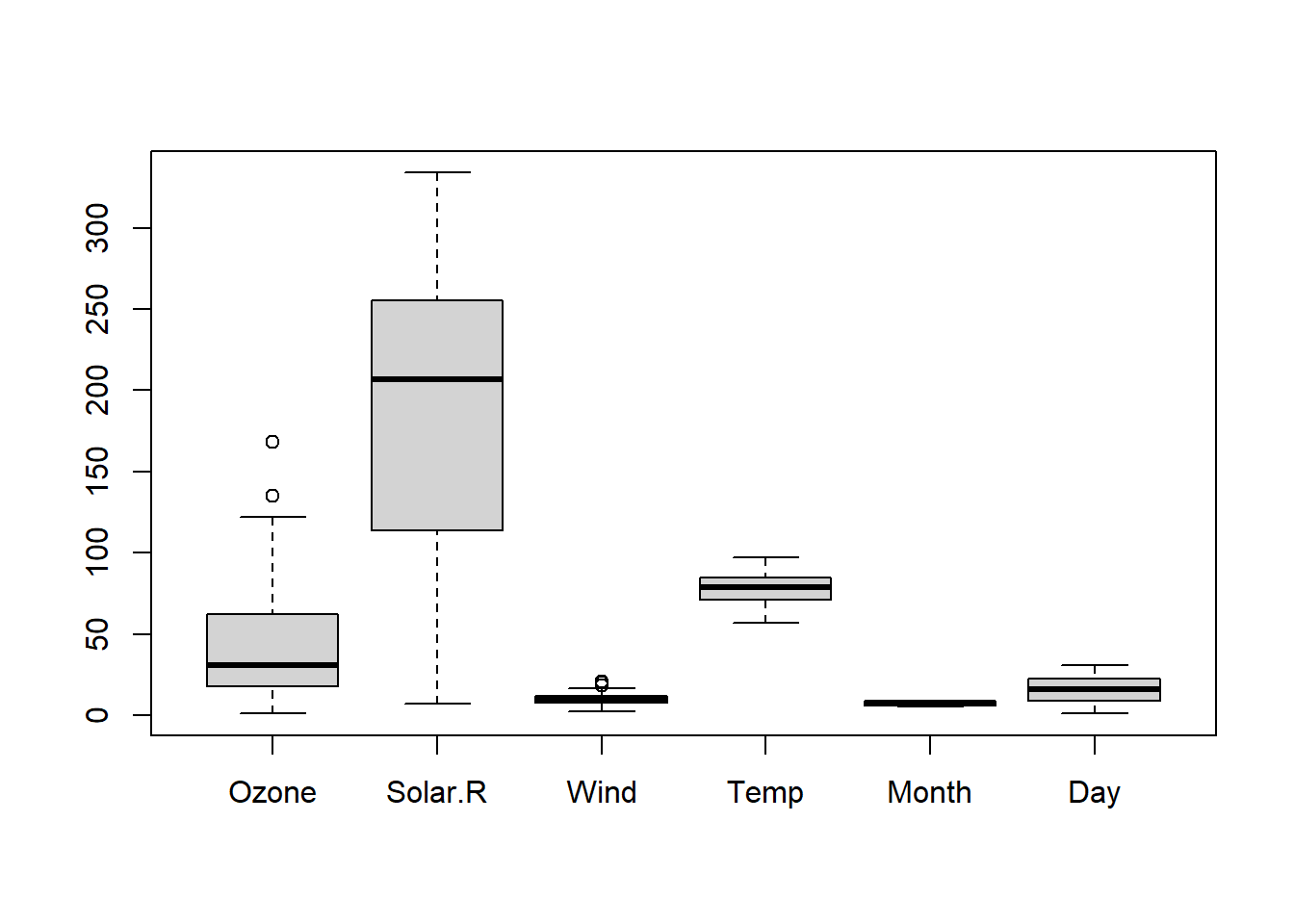
```Manage Outliers
Visualize data using boxplots, histograms, or scatter plots to detect outliers.
Consider using statistical methods or domain knowledge to handle outliers, such as winsorization or transformation.
```{r}
#| label: Boxplot of air wauality data set
#| fig-alt: "Boxplot of air wauality data set"

# Example: Visualize outliers using a boxplot
boxplot(airquality_clean)


# # Remove outliers from the 'income' variable
# airquality_clean <- airquality_clean %>%
#   filter(Ozone >= 0)
```
Correct Errors
Check for data entry errors and inconsistencies.
Use data validation rules or regular expressions to identify and correct errors.
Data Transformation
To make your data acceptable for analysis, you must shape and reformat it through data transformation. The following are a few excellent practices for R’s data transformation:
Use Tidy Data Principles
Follow the principles of tidy data, where each variable is a column, each observation is a row, and each type of observational unit is a table.
The
tidyrpackage provides functions likegather()andspread()for reshaping data.
```{r}
# # Example: Convert data from wide to long format
airquality_clean_long <- airquality_clean %>%
  gather(key = "Column_name", value = "value")

head(airquality_clean_long)
```Column_name <chr> | value <dbl> | |||
|---|---|---|---|---|
| 1 | Ozone | 41 | ||
| 2 | Ozone | 36 | ||
| 3 | Ozone | 12 | ||
| 4 | Ozone | 18 | ||
| 5 | Ozone | 23 | ||
| 6 | Ozone | 19 |
Apply Data Type Conversions
Ensure that variables have the correct data types (e.g., numeric, character, factor) for analysis.
Use functions like
as.numeric(),as.character(), oras.factor()to convert data types.
```{r}
# Example: Convert a variable to numeric
airquality_clean$Temp_numeric <- as.numeric(airquality_clean$Temp)

head(airquality_clean)
```Ozone <int> | Solar.R <int> | Wind <dbl> | Temp <int> | Month <int> | Day <int> | Temp_numeric <dbl> | |
|---|---|---|---|---|---|---|---|
| 1 | 41 | 190 | 7.4 | 67 | 5 | 1 | 67 |
| 2 | 36 | 118 | 8.0 | 72 | 5 | 2 | 72 |
| 3 | 12 | 149 | 12.6 | 74 | 5 | 3 | 74 |
| 4 | 18 | 313 | 11.5 | 62 | 5 | 4 | 62 |
| 7 | 23 | 299 | 8.6 | 65 | 5 | 7 | 65 |
| 8 | 19 | 99 | 13.8 | 59 | 5 | 8 | 59 |
Data Validation
To ensure that your processed data satisfies the criteria of your study, validation is a crucial stage in the data wrangling process. Here are a few guidelines for using R’s data validation features.
Perform Sanity Checks
- Check summary statistics, distributions, and relationships between variables to ensure they align with your expectations.
```{r}
# Example: Check summary statistics
summary(airquality_clean)
```
Ozone Solar.R Wind Temp
Min. : 1.0 Min. : 7.0 Min. : 2.30 Min. :57.00
1st Qu.: 18.0 1st Qu.:113.5 1st Qu.: 7.40 1st Qu.:71.00
Median : 31.0 Median :207.0 Median : 9.70 Median :79.00
Mean : 42.1 Mean :184.8 Mean : 9.94 Mean :77.79
3rd Qu.: 62.0 3rd Qu.:255.5 3rd Qu.:11.50 3rd Qu.:84.50
Max. :168.0 Max. :334.0 Max. :20.70 Max. :97.00
Month Day Temp_numeric
Min. :5.000 Min. : 1.00 Min. :57.00
1st Qu.:6.000 1st Qu.: 9.00 1st Qu.:71.00
Median :7.000 Median :16.00 Median :79.00
Mean :7.216 Mean :15.95 Mean :77.79
3rd Qu.:9.000 3rd Qu.:22.50 3rd Qu.:84.50
Max. :9.000 Max. :31.00 Max. :97.00 Validate Data Integrity
Verify that data transformations have not introduced errors.
Compare original and transformed data to identify discrepancies.
Document Your Steps
For reproducibility and collaboration, it’s essential to record your data manipulation procedures. To write a narrative that details the choices you made while handling the data, think about utilizing R Markdown or Jupyter Notebooks. Make your work accessible and understandable to others by using code comments, explanations, and visualizations.
Conclusion
A crucial first step in data analysis is data wrangling; by using R’s best practices, you can speed up the process and guarantee the accuracy of your findings. You may improve the efficiency of your data wrangling workflow and provide more reliable analyses by comprehending your data, putting effective cleaning and transformation strategies into practice, testing your findings, and documenting your approach.
Always tailor these best practices to your unique needs, keeping in mind that the individual methods and packages you use may vary depending on your dataset and research goals.